| Dataset Dimensions | |
|---|---|
| rows_number | columns_number |
| 3000 | 22 |
Communicating the Updated Analysis
Biagio Palese
The last step

We are at the end of our journey.. we finally reached the top
I know that

all of you feel better about R
We come a long way

Artwork by @allison_horst
Class Objective
- Show the additional analysis performed.
- Communicate the results of the updated data analysis.
Hotel Analysis Scenario
OptimaHotel Insights has been tasked by multiple hotel chains to develop a predictive model that can accurately forecast Average Daily Rates (ADR) based on various hotel features.
Updated ADR Analysis Deliverables
- Update the presentation to address the OptimaHotel Insights representatives feedback.
- Show the outcomes of the additional requested analyses from the OptimaHotel Insights representives.
Step 1: Exploring the Dataset
The hotel_data dataset used in this case study contains comprehensive information on various attributes and performance metrics of 3000 hotels across major U.S. cities.
It is meticulously curated1 to support predictive analyses focused on predicting and optimizing the average daily rate (ADR) for these properties.
This dataset includes realistic and detailed data, encompassing a wide range of features crucial for developing predictive pricing models.
| Dataset Glimpse | ||
|---|---|---|
| Column Name | Data Type | Example Values |
| id | numeric | 1, 2, 3 |
| num_rooms | numeric | 33, 71, 150 |
| location_quality | character | Excellent, Excellent, Good |
| star_rating | numeric | 1, 5, 3 |
| review_score | numeric | 1.84, 1.88, 2.93 |
| occupancy_rate | numeric | 71.65, 52.29, 97.43 |
| amenities_score | numeric | 3, 5, 1 |
| business_facilities | numeric | 0, 1, 1 |
| leisure_facilities | numeric | 1, 1, 1 |
| distance_to_city_center | numeric | 7.92, 4.85, 8.58 |
| average_daily_rate | numeric | 98.22, 98.73, 106.56 |
| city | character | Chicago, New York, Los Angeles |
| hotel_chain | character | Hilton, Hyatt, Marriott |
| month | numeric | 1, 5, 12 |
| season | character | Winter, Spring, Winter |
| number_of_bookings | numeric | 53, 61, 58 |
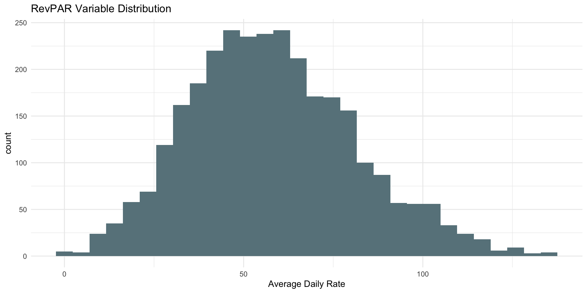
| revPAR | numeric | 70.37, 51.62, 103.82 |
| average_length_of_stay | numeric | 4.45, 3.09, 3.6 |
| competitors_average_price | numeric | 88.56, 84.46, 131.51 |
| transport_accessibility_score | numeric | 3.67, 6.3, 6.3 |
| customer_satisfaction_index | numeric | 81.57, 94.62, 91.12 |
| cancellation_rate | numeric | 0.01, 0.1, 0.14 |
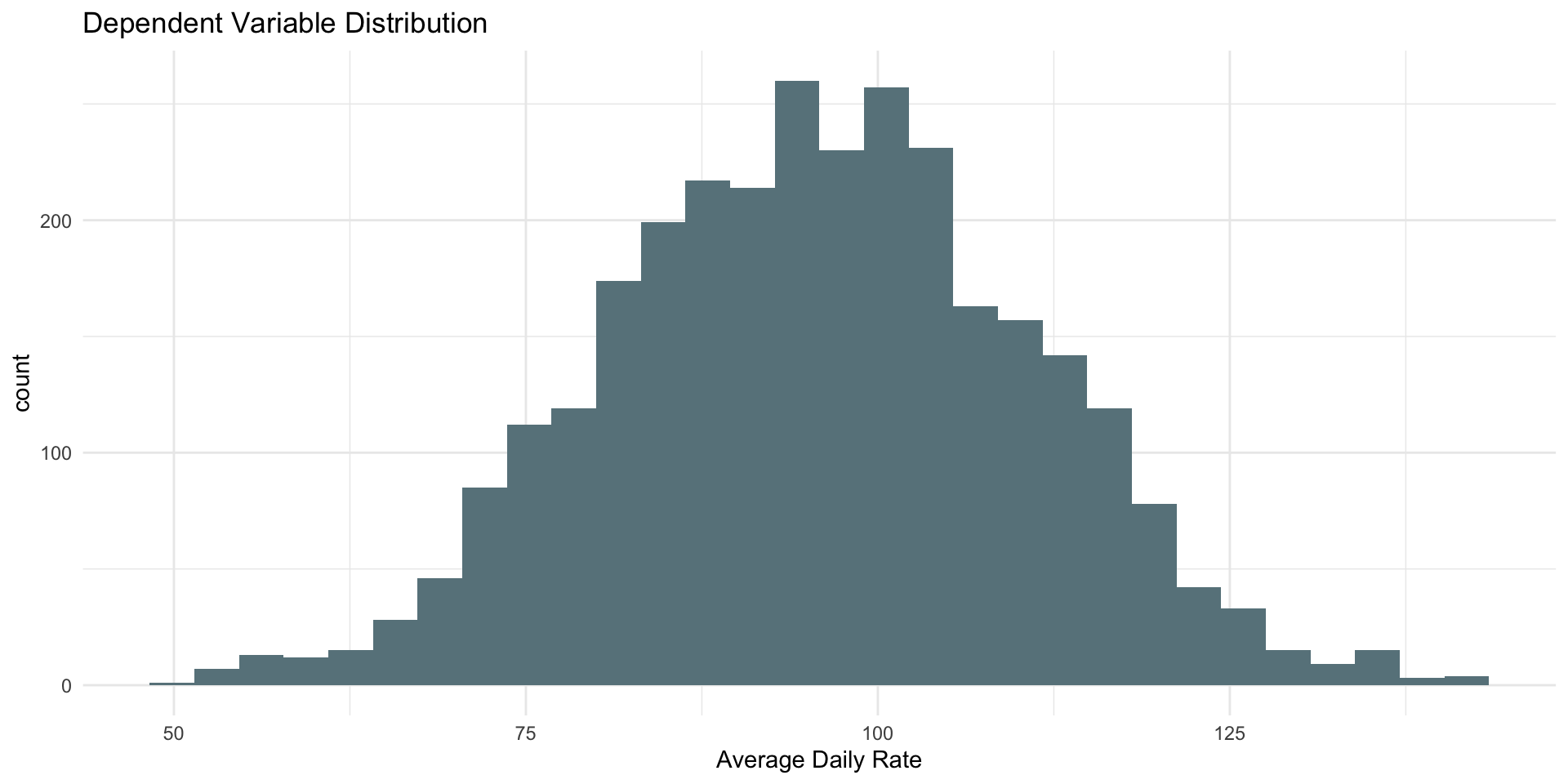
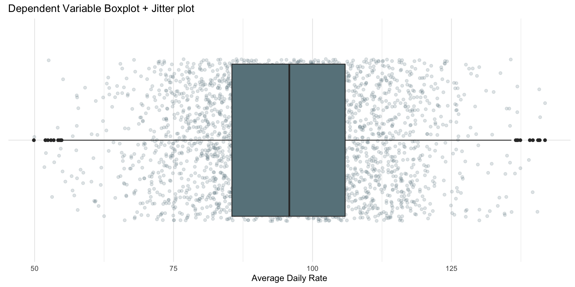
| ADR Descriptive Stats | ||||
|---|---|---|---|---|
| min_average_daily_rate | avg_average_daily_rate | median_average_daily_rate | max_average_daily_rate | sd_average_daily_rate |
| 49.87 | 95.87045 | 95.825 | 141.83 | 14.98696 |
| ADR Descriptive Stats by City | |||||
|---|---|---|---|---|---|
| city | min_average_daily_rate | avg_average_daily_rate | median_average_daily_rate | max_average_daily_rate | sd_average_daily_rate |
| Chicago | 53.45 | 96.02526 | 96.045 | 141.83 | 15.48101 |
| Los Angeles | 49.87 | 95.56752 | 95.160 | 135.78 | 14.67615 |
| Miami | 54.23 | 96.19310 | 96.105 | 139.10 | 14.19395 |
| New York | 57.49 | 95.71646 | 95.930 | 140.88 | 15.10470 |
| San Francisco | 51.98 | 95.88067 | 96.085 | 140.77 | 15.45662 |
| ADR Descriptive Stats by Hotel Chain | |||||
|---|---|---|---|---|---|
| hotel_chain | min_average_daily_rate | avg_average_daily_rate | median_average_daily_rate | max_average_daily_rate | sd_average_daily_rate |
| Hilton | 55.12 | 95.92 | 96.00 | 140.77 | 15.51 |
| Hyatt | 54.78 | 95.28 | 95.08 | 141.83 | 15.24 |
| InterContinental | 51.94 | 96.31 | 96.67 | 139.10 | 14.70 |
| Marriott | 57.47 | 95.87 | 96.32 | 140.88 | 14.52 |
| Sheraton | 49.87 | 96.01 | 95.93 | 139.65 | 14.98 |
Step 2: Manipulating the Data
Based on the above exploration the following minor manipulations1 are required:
Transformed month from numeric to factor
Step 3: Checking Correlations
Given that we are working on a new dataset and that we are not super familiar with hotel data, it is worth to take a look at the correlation of our numerical variables.
Correlation Matrix
| Correlation Matrix Arranged By ADR | ||||||||||||||||
|---|---|---|---|---|---|---|---|---|---|---|---|---|---|---|---|---|
| variables | number_of_bookings | num_rooms | star_rating | review_score | occupancy_rate | amenities_score | business_facilities | leisure_facilities | average_daily_rate | revPAR | average_length_of_stay | competitors_average_price | transport_accessibility_score | customer_satisfaction_index | cancellation_rate | miles_distance_to_city_center |
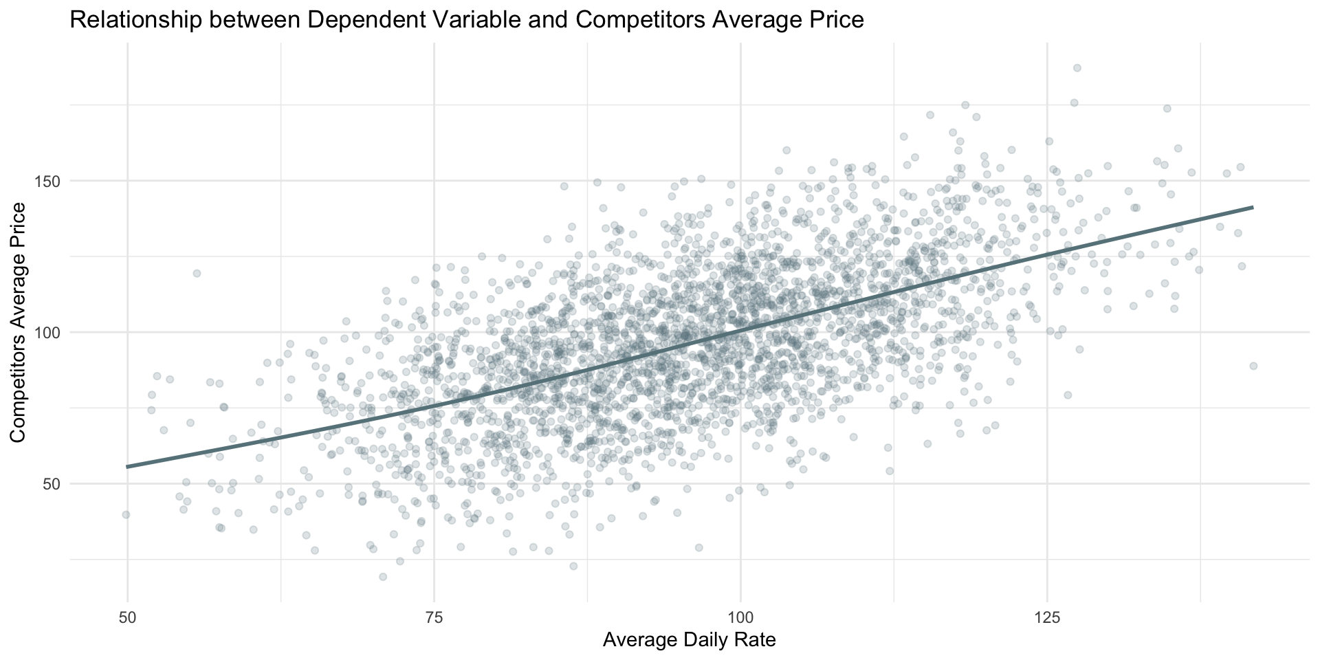
| average_daily_rate | 0.0274 | 0.0043 | 0.1443 | 0.0301 | 0.2323 | 0.0145 | 0.2832 | 0.4994 | 1.0000 | 0.5704 | -0.0028 | 0.5749 | -0.0041 | -0.0271 | 0.0105 | 0.0031 |
| competitors_average_price | 0.0047 | -0.0096 | 0.0878 | 0.0044 | 0.1385 | 0.0080 | 0.1251 | 0.2872 | 0.5749 | 0.3305 | 0.0074 | 1.0000 | -0.0087 | -0.0033 | 0.0163 | -0.0121 |
| revPAR | -0.0080 | 0.0071 | 0.0790 | 0.0221 | 0.9228 | 0.0000 | 0.1011 | 0.1582 | 0.5704 | 1.0000 | -0.0181 | 0.3305 | -0.0175 | -0.0023 | 0.0076 | 0.0003 |
| leisure_facilities | 0.0336 | -0.0099 | 0.0177 | 0.0034 | -0.0350 | 0.0122 | -0.0179 | 1.0000 | 0.4994 | 0.1582 | 0.0042 | 0.2872 | -0.0027 | -0.0247 | 0.0020 | -0.0020 |
| business_facilities | -0.0125 | -0.0061 | 0.0068 | -0.0195 | -0.0080 | -0.0383 | 1.0000 | -0.0179 | 0.2832 | 0.1011 | -0.0120 | 0.1251 | -0.0008 | 0.0062 | -0.0243 | 0.0100 |
| occupancy_rate | -0.0226 | 0.0065 | 0.0254 | 0.0148 | 1.0000 | -0.0052 | -0.0080 | -0.0350 | 0.2323 | 0.9228 | -0.0202 | 0.1385 | -0.0220 | 0.0076 | 0.0013 | -0.0005 |
| star_rating | 0.0138 | 0.0044 | 1.0000 | -0.0049 | 0.0254 | -0.0035 | 0.0068 | 0.0177 | 0.1443 | 0.0790 | -0.0243 | 0.0878 | 0.0094 | -0.0128 | 0.0085 | 0.0235 |
| review_score | 0.0129 | 0.0123 | -0.0049 | 1.0000 | 0.0148 | 0.0063 | -0.0195 | 0.0034 | 0.0301 | 0.0221 | -0.0317 | 0.0044 | -0.0135 | 0.0010 | -0.0464 | 0.0005 |
| number_of_bookings | 1.0000 | -0.0037 | 0.0138 | 0.0129 | -0.0226 | 0.0175 | -0.0125 | 0.0336 | 0.0274 | -0.0080 | 0.0183 | 0.0047 | -0.0121 | 0.0009 | -0.0113 | 0.0100 |
| amenities_score | 0.0175 | -0.0318 | -0.0035 | 0.0063 | -0.0052 | 1.0000 | -0.0383 | 0.0122 | 0.0145 | 0.0000 | -0.0304 | 0.0080 | -0.0131 | 0.0304 | -0.0188 | 0.0069 |
| cancellation_rate | -0.0113 | -0.0024 | 0.0085 | -0.0464 | 0.0013 | -0.0188 | -0.0243 | 0.0020 | 0.0105 | 0.0076 | 0.0056 | 0.0163 | -0.0037 | 0.0051 | 1.0000 | 0.0042 |
| num_rooms | -0.0037 | 1.0000 | 0.0044 | 0.0123 | 0.0065 | -0.0318 | -0.0061 | -0.0099 | 0.0043 | 0.0071 | -0.0222 | -0.0096 | 0.0135 | 0.0309 | -0.0024 | 0.0068 |
| miles_distance_to_city_center | 0.0100 | 0.0068 | 0.0235 | 0.0005 | -0.0005 | 0.0069 | 0.0100 | -0.0020 | 0.0031 | 0.0003 | -0.0263 | -0.0121 | 0.0089 | -0.0117 | 0.0042 | 1.0000 |
| average_length_of_stay | 0.0183 | -0.0222 | -0.0243 | -0.0317 | -0.0202 | -0.0304 | -0.0120 | 0.0042 | -0.0028 | -0.0181 | 1.0000 | 0.0074 | 0.0238 | -0.0063 | 0.0056 | -0.0263 |
| transport_accessibility_score | -0.0121 | 0.0135 | 0.0094 | -0.0135 | -0.0220 | -0.0131 | -0.0008 | -0.0027 | -0.0041 | -0.0175 | 0.0238 | -0.0087 | 1.0000 | -0.0210 | -0.0037 | 0.0089 |
| customer_satisfaction_index | 0.0009 | 0.0309 | -0.0128 | 0.0010 | 0.0076 | 0.0304 | 0.0062 | -0.0247 | -0.0271 | -0.0023 | -0.0063 | -0.0033 | -0.0210 | 1.0000 | 0.0051 | -0.0117 |
Step 4: Data Splitting
When it comes to supervised data modeling one of the most adopted method to evaluate multiple models is to split the data into a training set and a test set from the beginning.
Hotel train
| Training Dataset Dimensions | |
|---|---|
| rows_number | columns_number |
| 2192 | 22 |
Hotel test
| Test Dataset Dimensions | |
|---|---|
| rows_number | columns_number |
| 731 | 22 |
Step 5: Setting up the Recipes
Creating recipes is a critical step because it allows to define the model formula and specify any preprocessing steps to the original dataset.
Recipe 1
Recipe 2
Recipe 3
NEW: Recipe 4
recipe4 <- recipe(average_daily_rate ~ ., data = hotel_train)|>
  step_dummy(all_nominal_predictors()) |>
  step_interact(terms = ~cancellation_rate:number_of_bookings) |>
  step_interact(terms = ~occupancy_rate:number_of_bookings) |>
  step_interact(terms= ~transport_accessibility_score:miles_distance_to_city_center)
Step 6: Specifying the Models
We specify five models using parsnip:
a
lmenginelinear regression;a
glmnetenginelasso regression1;a
glmentengineridge regression(NEW);a
rpartenginedecision tree(NEW);a
rangerenginerandom forest(NEW)2.
Model 1
Model 2
NEW: Model 3
NEW: Model 4
NEW: Model 5
Step 7: Fitting Models using Workflows
Next, we fit the models to the hotel_train dataset, so that we can compare their predictions performance on hotel_test.
This is accomplished by embedding the model specifications within workflows that also incorporate our preprocessing recipes.
I will only use recipe 2, 3 & 4 for my workflow based on the results of the first presentation.
Step 8: Making Predictions
Then we use the models built on the training set to make predictions on our test set.
By doing so we will have both the actual values and the predicted values and we can assess the model performance.
Lasso recipe 4 model actual ADR values vs predicted
| ADR actual vs predicted values | |
|---|---|
| adr | pred_adr |
| 84.520000 | 85.882901 |
| 79.160000 | 80.365714 |
| 107.740000 | 109.831862 |
| 104.800000 | 100.121869 |
| 97.880000 | 100.510787 |
| 126.980000 | 125.906419 |
| 76.970000 | 77.913506 |
| 101.360000 | 98.790749 |
| 93.440000 | 91.641639 |
| 119.410000 | 120.602377 |
Step 9: Assess Models Performance
While seeing the predictions next to the actual values can already provide some insights on the goodness of the model.
In regression analysis, model performance is evaluated using specific metrics that quantify the model’s accuracy and ability to generalize.
Three fundamental metrics are Root Mean Squared Error (RMSE), Mean Absolute Error (MAE), and R-squared (R²).
| Full Metrics Table | ||
|---|---|---|
| .metric | .estimate | model |
| mae | 2.9542 | reg_model_recipe3 |
| mae | 2.9590 | reg_model_recipe4 |
| mae | 2.9813 | lasso_model_recipe4 |
| mae | 2.9816 | lasso_model_recipe3 |
| mae | 4.6031 | ridge_model_recipe4 |
| mae | 4.7870 | ridge_model_recipe3 |
| mae | 6.3418 | rf_model_recipe4 |
| mae | 6.4312 | rf_model_recipe3 |
| mae | 7.8728 | dt_model_recipe3 |
| mae | 7.8728 | dt_model_recipe4 |
| mae | 7.9723 | lasso_model_recipe2 |
| mae | 7.9748 | reg_model_recipe2 |
| mae | 7.9845 | ridge_model_recipe2 |
| mae | 8.1338 | rf_model_recipe2 |
| mae | 8.9367 | dt_model_recipe2 |
| rmse | 4.1066 | reg_model_recipe3 |
| rmse | 4.1073 | reg_model_recipe4 |
| rmse | 4.1121 | lasso_model_recipe4 |
| rmse | 4.1123 | lasso_model_recipe3 |
| rmse | 5.8296 | ridge_model_recipe4 |
| rmse | 6.0467 | ridge_model_recipe3 |
| rmse | 7.9047 | rf_model_recipe4 |
| rmse | 7.9884 | rf_model_recipe3 |
| rmse | 9.7966 | reg_model_recipe2 |
| rmse | 9.8012 | lasso_model_recipe2 |
| rmse | 9.8104 | ridge_model_recipe2 |
| rmse | 9.8150 | dt_model_recipe3 |
| rmse | 9.8150 | dt_model_recipe4 |
| rmse | 10.0920 | rf_model_recipe2 |
| rmse | 11.0944 | dt_model_recipe2 |
| rsq | 0.3721 | dt_model_recipe2 |
| rsq | 0.4772 | rf_model_recipe2 |
| rsq | 0.5067 | reg_model_recipe2 |
| rsq | 0.5068 | dt_model_recipe3 |
| rsq | 0.5068 | dt_model_recipe4 |
| rsq | 0.5068 | lasso_model_recipe2 |
| rsq | 0.5071 | ridge_model_recipe2 |
| rsq | 0.7105 | rf_model_recipe3 |
| rsq | 0.7276 | rf_model_recipe4 |
| rsq | 0.8234 | ridge_model_recipe3 |
| rsq | 0.8363 | ridge_model_recipe4 |
| rsq | 0.9133 | reg_model_recipe4 |
| rsq | 0.9133 | reg_model_recipe3 |
| rsq | 0.9145 | lasso_model_recipe3 |
| rsq | 0.9145 | lasso_model_recipe4 |
By looking at the metrics table
recipe 3 lassois still the best model (recipe4 is only slightly better but more complex).We excluded the
recipe 3 and 4 regressionmodel because of a warning highlighting issues during its fit.Adding complexity (interactions terms & more advanced models) doesn’t always pay off.
Step 10: Visualizing Prediction Results
Visualizing the prediction results can provide additional insights into model performance.
You should plot the predicted vs actual values and the residuals to visually assess how well the model is capturing the underlying relationship in the data.
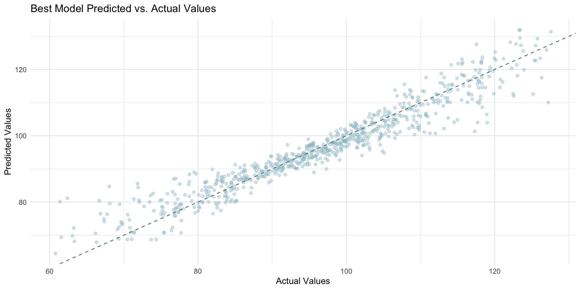
Adding interaction terms (recipe4 lasso) didn’t result in the expected improvements in the residuals.
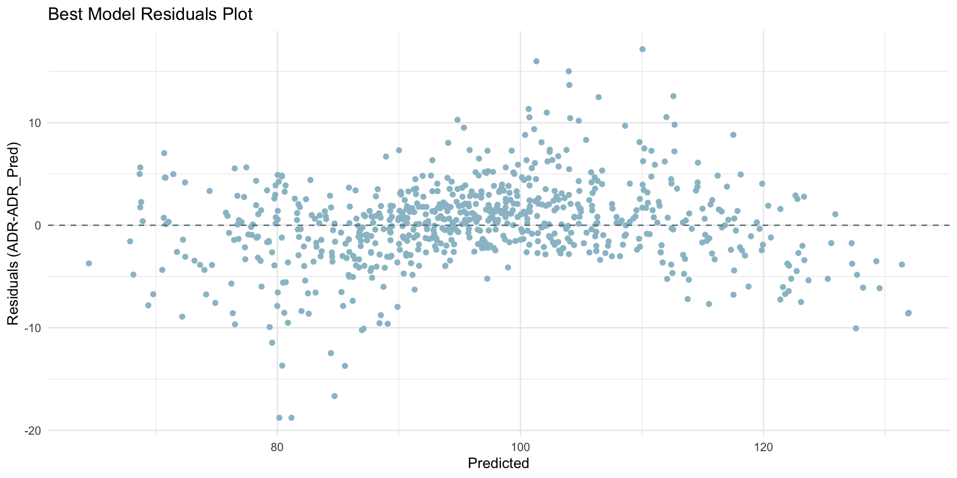
While the random forest unperformed in terms of prediction accuracy, our intuition to use it to address the slight non-linearity of our residuals was correct.
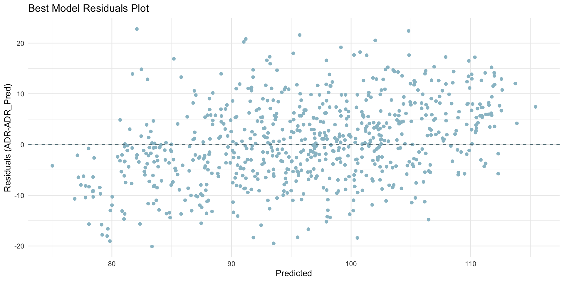
After adding interactions terms, we could go back and try some variable transformations on the most relevant variables. However, we will stop here for this demo.
Visual interpretations provide valuable insights into model performance but should be complemented with quantitative metrics (like RMSE, MAE and R²) for a comprehensive evaluation.
The plots help identifying patterns or biases not immediately apparent from numerical metrics alone.
Step 11: Model Interpretation
Given that I have already shown how to interpret recipe3 lasso regression, I want to use this updated presentation to interpret the linear regression and decision tree models (ridge is identical to lasso and random forest was beyond the scope of the class).
Zero Coefficients Variables do not have a statistically significant linear relationship with ADR after accounting for other variables and the regularization penalty.
| Removed Predictors | ||
|---|---|---|
| term | estimate | penalty |
| num_rooms | 0.000000 | 0.100000 |
| number_of_bookings | 0.000000 | 0.100000 |
| average_length_of_stay | 0.000000 | 0.100000 |
| transport_accessibility_score | 0.000000 | 0.100000 |
| miles_distance_to_city_center | 0.000000 | 0.100000 |
| city_Los.Angeles | 0.000000 | 0.100000 |
| city_Miami | 0.000000 | 0.100000 |
| city_New.York | 0.000000 | 0.100000 |
| city_San.Francisco | 0.000000 | 0.100000 |
| hotel_chain_Hyatt | 0.000000 | 0.100000 |
| hotel_chain_Marriott | 0.000000 | 0.100000 |
| hotel_chain_Sheraton | 0.000000 | 0.100000 |
| month_X2 | 0.000000 | 0.100000 |
| month_X3 | 0.000000 | 0.100000 |
| month_X4 | 0.000000 | 0.100000 |
| month_X5 | 0.000000 | 0.100000 |
| month_X7 | 0.000000 | 0.100000 |
| month_X12 | 0.000000 | 0.100000 |
| season_Spring | 0.000000 | 0.100000 |
| season_Summer | 0.000000 | 0.100000 |
| season_Winter | 0.000000 | 0.100000 |
Non-Zero Coefficients Variables are influencing factors for ADR and should be considered in pricing strategies.
| Included Predictors | ||
|---|---|---|
| term | estimate | penalty |
| (Intercept) | 83.397249 | 0.100000 |
| star_rating | 0.172368 | 0.100000 |
| review_score | 0.106223 | 0.100000 |
| occupancy_rate | −1.143629 | 0.100000 |
| amenities_score | 0.015145 | 0.100000 |
| business_facilities | 1.712883 | 0.100000 |
| leisure_facilities | 2.758931 | 0.100000 |
| revPAR | 1.243878 | 0.100000 |
| competitors_average_price | 0.052473 | 0.100000 |
| customer_satisfaction_index | −0.004735 | 0.100000 |
| cancellation_rate | −0.576860 | 0.100000 |
| location_quality_Excellent | 1.881180 | 0.100000 |
| location_quality_Good | 0.948190 | 0.100000 |
| location_quality_Poor | −0.762115 | 0.100000 |
| hotel_chain_InterContinental | 0.000765 | 0.100000 |
| month_X6 | 0.026898 | 0.100000 |
| month_X8 | −0.005338 | 0.100000 |
| month_X9 | −0.010730 | 0.100000 |
| month_X10 | −0.220501 | 0.100000 |
| month_X11 | 0.056927 | 0.100000 |
Intercept: $83.4 represent the expected ADR when the categorical predictors are in their baseline category (the first value in alphabetical order) and the numerical predictors are zero or at their lowest practical/observed levels.
| Intercept Only Table | |
|---|---|
| term | estimate |
| (Intercept) | 83.397249 |
Star Rating: For one additional star, ADR increases by approximately $0.171, assuming all other variables remain constant.
This means that moving from 1-star to a 5-star hotel, which is an increase of 4 stars, would lead to an estimated increase of 0.171 x 4 = $0.684 in ADR1.
| Star Rating Only Table | |
|---|---|
| term | estimate |
| star_rating | 0.172368 |
Review Score: For one point increase in the review score (on a scale of 1 to 5), ADR increases by $0.106 given all other variables staying constant.
| Review Score Only Table | |
|---|---|
| term | estimate |
| review_score | 0.106223 |
This shows the value customers place on higher-rated hotels, which can command higher prices but the impact is surprisingly small.
Occupancy Rate: For one percentage point increase in occupancy rate, ADR decreases by $1.14. Surprisingly, higher occupancy rates do not correspond with higher ADR.
| Occupancy Rate Only Table | |
|---|---|
| term | estimate |
| occupancy_rate | −1.143629 |
It’s possible that in an effort to maintain high occupancy levels, hotels might be underpricing their rooms, thus not maximizing potential revenue.
Business Facilities & Leisure Facilities: Hotels with business and leisure facilities can charge an additional $1.71 and $2.76, respectively, on ADR.
| Business Facilities & Leisure Facilities Only Table | |
|---|---|
| term | estimate |
| business_facilities | 1.712883 |
| leisure_facilities | 2.758931 |
However, these amenities impact does not seem substantial at first glance, particularly when considering the potential costs associated with maintaining them (e.g., might test their interaction).
RevPAR (Revenue per Available Room): This variable is an important hospitality metrics. RevPAR combines the effects of room rates and occupancy levels. For one dollar increase in RevPAR, ADR increases by $1.24.
| RevPAR Only Table | |
|---|---|
| term | estimate |
| revPAR | 1.243878 |
Competitors Average Price: For one dollar increase in competitors' average prices, ADR increases by only $0.0525.
| Competitors Average Price Only Table | |
|---|---|
| term | estimate |
| competitors_average_price | 0.052473 |
The strategy of not matching the price increases fully could reflect a positioning approach where hotels aim to offer slightly lower prices to attract price-sensitive customers or to increase market share by becoming a more economical option within their competitive set.
Customer Satisfaction Index: For every one-unit increase in the customer satisfaction index, ADR decreases by approximately $0.005, assuming other factors remain constant.
| Customer Satisfaction Index Only Table | |
|---|---|
| term | estimate |
| customer_satisfaction_index | −0.004735 |
The negative coefficient suggests a potential under utilization of customer satisfaction. Thus, increases in customer satisfaction do not translate into higher ADR.
Cancellation Rate: For each percentage point increase in cancellation rates, ADR decreases by $0.570.
| Cancellation Rate Only Table | |
|---|---|
| term | estimate |
| cancellation_rate | −0.576860 |
While this drop in price can mitigate the risk of empty rooms, it also suggests potential revenue losses or instability in booking patterns.
Location Quality: Being in an Excellent location increases the ADR by $1.89, while being in a Good location increases it by $0.952, compared to our baseline, Average location.
| Location Quality Only Table | |
|---|---|
| term | estimate |
| location_quality_Excellent | 1.881180 |
| location_quality_Good | 0.948190 |
| location_quality_Poor | −0.762115 |
Being in a Poor location decreases it by $0.755 compared to Average. Hotels are clearly underselling their premium locations.
Linear Regression Model Interpretation
Before interpreting the individual variables, let’s break down the meaning of each column available in a linear regression results table:
Estimate:
Represents the average change in the dependent variable (ADR) for a one-unit increase in the independent variable, holding all other variables constant.
The value indicates the magnitude of the impact.
The sign indicates the direction of the impact.
Standard Error (std.error):
Reflects the variability or uncertainty of the estimated coefficient.
Smaller values indicate more precise estimates.
Statistic:
Also known as the t-value, this is the ratio of the estimate to its standard error.
Larger absolute values indicate that the variable is likely to be statistically significant.
p-value:
Indicates whether the variable is statistically significant.
Typically, a p-value below 0.05 means the variable has a significant relationship with the dependent variable.
Intercept:
When the categorical predictors are in their baseline category (the first value in alphabetical order) and the numerical are at zero or at their lowest practical/observed levels (e.g., revPAR = 0, competitors’ price = 0, baseline location quality = average, etc.), the predicted ADR is $53.44.
| Intercept Only Table | ||||
|---|---|---|---|---|
| term | estimate | std.error | statistic | p.value |
| (Intercept) | 53.4413 | 1.0742 | 49.7477 | 0.0000 |
revPAR:
For every 1 dollar increase in revPAR, the ADR increases by $0.26, assuming all other variables remain constant.
Significance: With a p-value of < 0.05, this relationship is statistically significant.
| RevPAR Only Table | ||||
|---|---|---|---|---|
| term | estimate | std.error | statistic | p.value |
| revPAR | 0.2580 | 0.0099 | 26.1377 | 0.0000 |
Competitors’ Average Price:
For every 1 dollar increase in competitors’ average price, ADR increases by $0.23, holding all else constant.
Significance: This is a strong, statistically significant predictor of ADR.
| Competitors Average Price Only Table | ||||
|---|---|---|---|---|
| term | estimate | std.error | statistic | p.value |
| competitors_average_price | 0.2328 | 0.0088 | 26.3102 | 0.0000 |
Star Rating:
For every one-star increase in the hotel’s rating, ADR increases by $0.94, assuming all other variables remain constant.
Significance: This is a strong, statistically significant predictor of ADR.
| Star Rating Only Table | ||||
|---|---|---|---|---|
| term | estimate | std.error | statistic | p.value |
| star_rating | 0.9389 | 0.1827 | 5.1376 | 0.0000 |
Location Quality: Hotels with an “Excellent” and “Good” location have a positive impact on ADR that is, on average, respectively 5.89 and 2.93 dollars higher than hotels with an “Average” location (the baseline category). While hotels with a “Poor” location have an ADR that is 1.50 dollars lower than those with an “Average” location, on average.
| Location Quality Only Table | ||||
|---|---|---|---|---|
| term | estimate | std.error | statistic | p.value |
| location_quality_Excellent | 5.8876 | 0.6001 | 9.8104 | 0.0000 |
| location_quality_Good | 2.9307 | 0.4929 | 5.9462 | 0.0000 |
| location_quality_Poor | −1.4989 | 0.7373 | −2.0330 | 0.0422 |
All three are statistically significant predictors of ADR.
Seasons:
The ADR for Spring (15 cents) and Winter (10 cents) is, on average, higher than in the baseline season (Fall). While the ADR for Summer is, on average, $0.94 lower than in the Fall.
| Location Quality Only Table | ||||
|---|---|---|---|---|
| term | estimate | std.error | statistic | p.value |
| season_Spring | 0.1534 | 0.5768 | 0.2660 | 0.7903 |
| season_Summer | −0.9380 | 0.5762 | −1.6278 | 0.1037 |
| season_Winter | 0.1009 | 0.5689 | 0.1774 | 0.8592 |
However, these results are not statistically significant (p > 0.05).
Decision Tree Interpretation
Decision tree are easier to interpret when you visualize them. See our decision tree for recipe2:
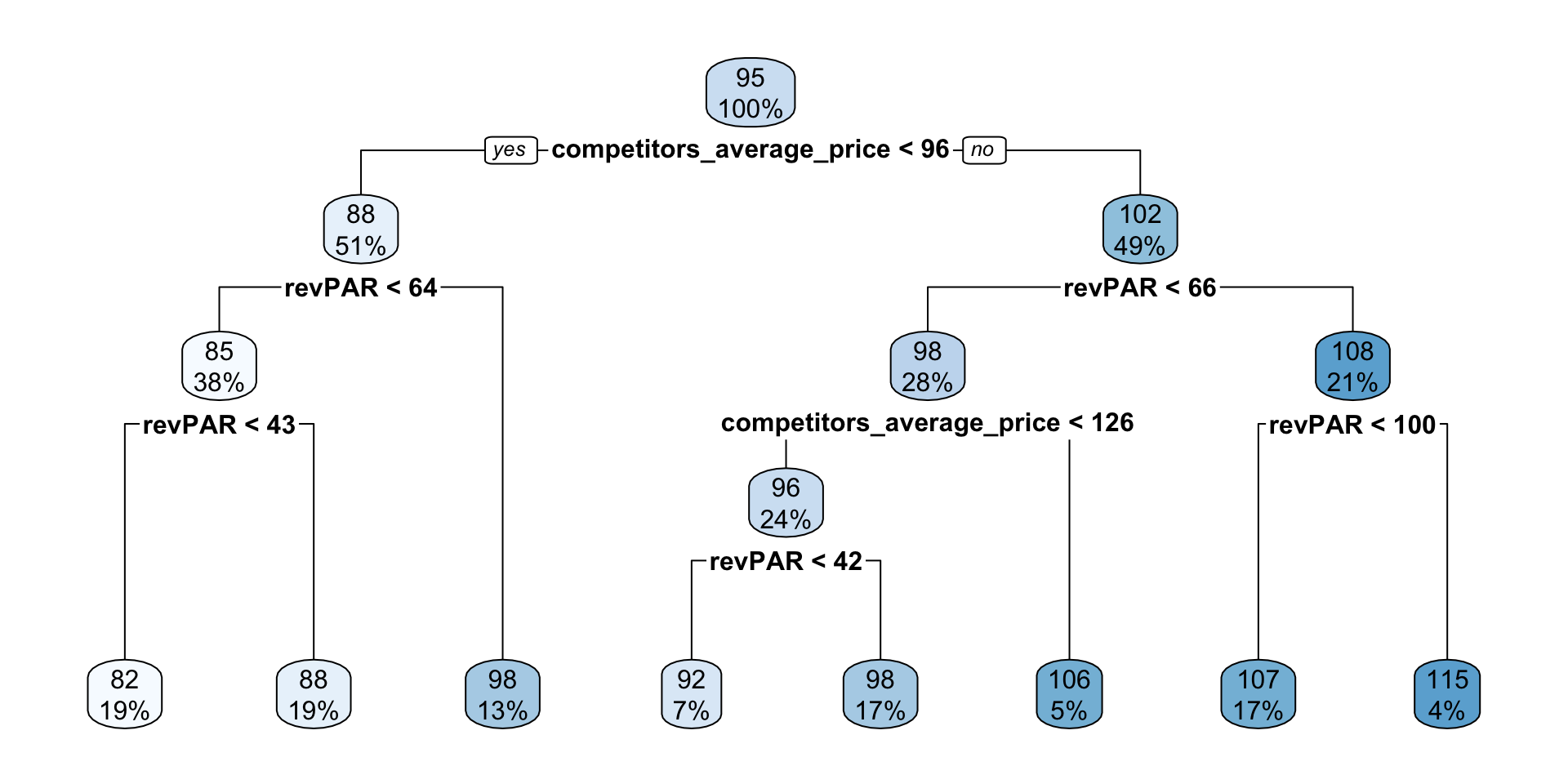
The following elements are key when interpreting tree based model results:
Nodes:
Decision Nodes: Represent a split in the data based on a condition (e.g.,
competitors_average_price < 96).Terminal Nodes (Leaves): Represent the end of a branch, containing the predicted value for a subset of the data.
Splits:
A split occurs when the tree partitions the data based on a predictor variable (
competitors_average_price,revPAR).Conditions at each split direct the data into smaller groups for improved homogeneity.
Branches:
Left Branch: Indicates that the condition at the split is satisfied (e.g.,
competitors_average_price < 96).Right Branch: Indicates the condition is not satisfied (e.g.,
competitors_average_price >= 96).
Predictions:
Each terminal node provides a predicted value for ADR.
These predictions are based on the characteristics of the subset of data reaching the node.
Proportions:
- Each terminal node also shows the percentage of data points in that node relative to the total dataset.
One more time..

The sky is the limit if you become an